Titanic - Machine Learning from Disaster

The Titanic: Machine Learning from Disaster project on Kaggle is a popular data science competition. The objective is to develop a predictive model that determines whether a given passenger survived the Titanic disaster. This is achieved by analyzing a dataset that includes variables such as the passenger’s age, sex, fare, cabin, embarkation point, among others.

Since this is my first project using Artificial Intelligence, I wanted to see how far I could go without the need for a specific tutorial or any external help. Throughout the process, I learned about statistics and various AI models that could assist me with this task. Here is how it went:

This competition presents two datasets containing passenger information from the historic RMS Titanic:

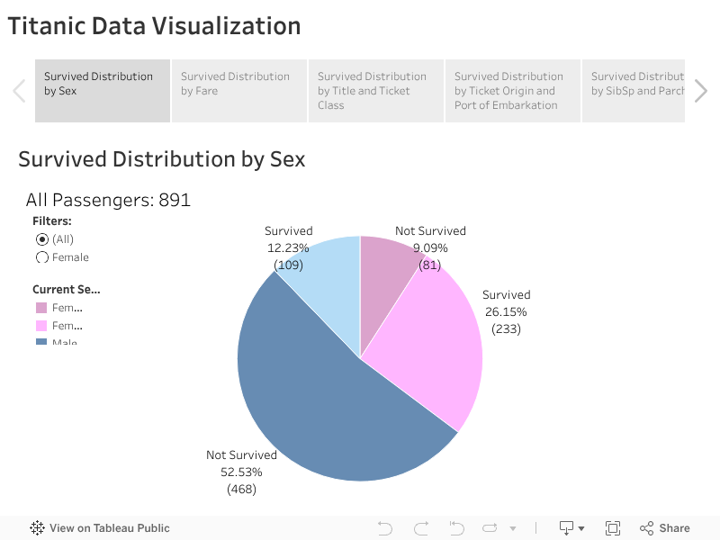
train.csv: Contains details for 891 passengers with survival outcomes:

PassengerId	Survived	Pclass	Name	Sex	Age	SibSp	Parch	Ticket	Fare	Cabin	Embarked
1	0	3	Braund, Mr. Owen Harris	male	22.0	1	0	A/5 21171	7.2500	NaN	S
2	1	1	Cumings, Mrs. John Bradley (Florence Briggs Thayer)	female	38.0	1	0	PC 17599	71.2833	C85	C
3	1	3	Heikkinen, Miss. Laina	female	26.0	0	0	STON/O2. 3101282	7.9250	NaN	S
...	...	...	...	...	...	...	...	...	...	...	...
889	1	1	Behr, Mr. Karl Howell	male	26.0	0	0	111369	30.0000	C148	C
890	1	1	Behr, Mr. Karl Howell	male	26.0	0	0	111369	30.0000	C148	C
891	0	3	Dooley, Mr. Patrick	male	32.0	0	0	370376	7.7500	NaN	Q

test.csv: Contains 418 additional passengers data without survival outcomes:

PassengerId	Pclass	Name	Sex	Age	SibSp	Parch	Ticket	Fare	Cabin	Embarked
892	3	Kelly, Mr. James	male	34.5	0	0	330911	7.8292	NaN	Q
893	3	Wilkes, Mrs. James (Ellen Needs)	female	47.0	1	0	363272	7.0000	NaN	S
894	2	Myles, Mr. Thomas Francis	male	62.0	0	0	240276	9.6875	NaN	Q
...	...	...	...	...	...	...	...	...	...	...
1307	3	Saether, Mr. Simon Sivertsen	male	38.5	0	0	SOTON/O.Q. 3101262	7.2500	NaN	S
1308	3	Ware, Mr. Frederick	male	NaN	0	0	359309	8.0500	NaN	S
1309	3	Peter, Master. Michael J	male	NaN	1	1	2668	22.3583	NaN	C

Before diving into data analysis, it's crucial to first ensure the quality of our data. Higher-quality data leads to more reliable and insightful conclusions. Our dataset contains some missing data points, leaving the values for those entries unknown. This could be attributed to either the information being lost or not adequately collected.

First, let's import all the libraries we'll be using in this demonstration:

        
import pandas as pd #For Data Manipulation
import numpy as np #For Numerical Operations 
from sklearn.model_selection import train_test_split #To Split our dataset for training and validation purposes
from sklearn.metrics import mean_absolute_error, r2_score, mean_squared_error #To evaluate our model
from catboost import CatBoostRegressor #This is to create our Machine Learning model
      

Now, let's check which values are missing in our dataset by using pandas with the following python code:

        
#Reading CSV file
df = pd.read_csv('train.csv')

print(df.isnull().sum())
      

Which results on the following outcome:

        PassengerId      0 
        Survived         0
        Pclass           0
        Name             0
        Sex              0
        Age            177
        SibSp            0
        Parch            0
        Ticket           0
        Fare             0
        Cabin          687
        Embarked         2
        dtype: int64
      

We can see that the Cabin, Age, and Embarked sections contain missing data. Of the 891 data points in our dataset, 687 entries in the Cabin column are missing. Since this column doesn't really contribute much valuable information, we can go ahead and drop it. These missing values don’t offer any useful patterns for the model to learn from.

        
#Dropping cabin column // # Setting inplace=True applies the change directly to the existing DataFrame
df.drop(columns=['Cabin'], inplace=True)
      

For the Embarked section, we'll fill the two missing entries with the mode, since it's just a couple of values, using the most frequent category should work just fine.

        
#Calculating mode for Embarked Column and replacing missing values

print(df['Embarked'].value_counts()) #This shows us the value 'S' is the most repeated one
df['Embarked'] = df['Embarked'].fillna('S')
      

Now, let’s take a look at how our dataset is shaping up in terms of missing values.

        
        PassengerId      0
        Survived         0
        Pclass           0
        Name             0
        Sex              0
        Age            177
        SibSp            0
        Parch            0
        Ticket           0
        Fare             0
        Embarked         0
        dtype: int64
      

The Age column contains 177 missing values, to address this, we'll create a predictive model to estimate the missing ages. Why are we doing this?: The Age data could indicate underlying patterns worth investigating. However, before modeling, it's important to carry out feature selection to determine which variables are most relevant.

Let’s review the dataset's columns:
- PassengerId: This serves merely as an index and isn't necessary for our analysis at this stage.
- Survived: Our target variable for classification. Fortunately, it’s already well-formatted thanks to Kaggle’s preprocessing.
- Pclass: Represents ticket class, and it’s properly structured and ready for use.
- Name: While this field may not seem useful initially, it includes each passenger's title (e.g., Mr., Mrs., Miss). We can extract these titles into a new feature column called Title, which may offer valuable insights. Let's see how to extract this information:

  
#Adding new column 'Title'

pd.set_option('display.max_rows', None) #Used to display all the rows in our dataframe, this way we can explore it better

df['Title'] = None #Setting this column to none will help us filter the data by doing the following for each title we find:

df['Title'] = df['Name'].str.extract('(Mr\.)')
print(df['Title'].value_counts()) #Let's see how many values we were able to filter so far
print(df['Title'].isnull().value_counts()) #Let's see how many values on our new title column are empty

#This process was repeteated multiple times until we got the following filter: 
df['Title'] = df['Name'].str.extract(
'(Mr\.|Mrs\.|Miss|Dr\.|Master\.|Rev\.|Col\.|Major\.|Mlle\.|Jonkheer\.|Countess\. of|Mme\.|Don\.|Mme\.|Ms\.|Lady\.|Sir\.|Capt\.)'
)
print(df['Title'].value_counts()) 
print(df['Title'].isnull().value_counts()) #We should not have any null values left

df['Title'] = df['Title'].str.replace('.','') #Just taking out the '.' to make the column look better

- Sex: This feature is already properly formatted and ready for use.
- Age: This will serve as the target variable for our first predictive model.
- SibSp: Already clean and formatted correctly.
- Parch: No formatting issues, this column is good to go.
- Ticket: This column poses some challenges. Many of the entries appear inconsistent or unstructured, making it difficult to extract meaningful patterns. We'll attempt to clean and standardize this data by applying the same filtering techniques used earlier(It would have been easier to create a function to filter the data in stages, but I realized that halfway through writing the code. Lesson learned):

#Let's see if the data can be grouped and how is grouped
print('Initial Ticket Groups: \n',df['Ticket'].value_counts())


# Some entries contain purely numeric values, while others mix letters and numbers.
# Let's create a filter to isolate the entries with numeric-only values.
booleanMaskForNumbers = pd.to_numeric(df['Ticket'],errors='coerce').notna()

#This will show us the tickets that are only numbers
print('Numeric Tickets: \n', df.loc[booleanMaskForNumbers,['Ticket']].count())


#Let's begin filtering the data by creating a new column called 'NewTicket' with the information for the numeric tickets we just found

df['NewTicket'] = None
df.loc[booleanMaskForNumbers,['NewTicket']] = 'NUMERIC-TICKETS'

print('NewTicket Value counts: \n',df['NewTicket'].count()) #Let's see how many of the values on our new column are not empty


# Now, we will create a new filter for null values (values that have not been filtered yet), to avoid redefining the variable
# each time the dataframe changes, we will create a function that will create a boolean mask each time is called. 
# The function will have a reverse argument which will do the opposite

def get_unfiltered_values (reverse=False):
    if reverse == False:
        booleanMaskForNullValues = df['NewTicket'].isnull()
    else:
        booleanMaskForNullValues = ~df['NewTicket'].isnull()
    return booleanMaskForNullValues


# Now we can begin to filter the rest of the data in our ticket column, let's create another function that will print the
# remaining values that need to be filtered:
# The function will have a reverse argument which will do the opposite

def show_unfiltered_values(reverse=False):
    if reverse == False:
        print('Unfiltered values: \n',df.loc[get_unfiltered_values(),['Ticket','NewTicket']]) 
        #We are printing 'NewTicket' just to verify values are nulll
    else:
        print('Filtered values: \n', df.loc[get_unfiltered_values(reverse=True),['Ticket','NewTicket']])
    
show_unfiltered_values()

#tempBooleanMask will serve as a temporary mask for the letters and sequence of letters that need to be filtered

# 'PC' Categorical Value:

tempBooleanMask = df['Ticket'].str.contains('PC',case=False)

df.loc[get_unfiltered_values() & tempBooleanMask, 'NewTicket'] = 'PC'

show_unfiltered_values(reverse=False)


# 'SC/PARIS' Categorical Value: 

tempBooleanMask = df['Ticket'].str.contains('PARIS', case=False )
df.loc[get_unfiltered_values() & tempBooleanMask, 'NewTicket'] = 'SC/PARIS'


# 'CA' Categorical Value:

tempBooleanMask = df['Ticket'].str.contains('C', case=False ) & (
    df['Ticket'].str.contains('C',case=False)
) & (
    df['Ticket'].str.contains('A',case=False)
) & (
    ~(df['Ticket'].str.contains('S',case=False))
)

df.loc[get_unfiltered_values() & tempBooleanMask, 'NewTicket'] = 'CA'


# 'STON/02' Categorical Value:

tempBooleanMask = df['Ticket'].str.contains('SOTON', case=False )& (
    ~df['Ticket'].str.contains('C',case=False)
    ) | (
        df['Ticket'].str.contains('STON', case= False)
        )


df.loc[get_unfiltered_values() & tempBooleanMask, 'NewTicket'] = 'STON/02'



# 'SOC' Categorical Value:

tempBooleanMask = df['Ticket'].str.contains('S', case= False) & (
    df['Ticket'].str.contains('O',case=False)) & (
        df['Ticket'].str.contains('C',case=False)) & (
            ~df['Ticket'].str.contains('A|W',case=False)
        )
 
df.loc[get_unfiltered_values() & tempBooleanMask, 'NewTicket'] = 'SOC'



# 'SOPP' Categorical Value:


tempBooleanMask = df['Ticket'].str.contains('S',case= False) & (
    df['Ticket'].str.contains('O',case= False)
    ) & (
        df['Ticket'].str.contains('P',case= False)
        )


df.loc[get_unfiltered_values() & tempBooleanMask, 'NewTicket'] = 'SOPP'



# 'A5/A4' Categorical Value:

tempBooleanMask = df['Ticket'].str.contains('A') & df['Ticket'].str.contains('5') 

df.loc[get_unfiltered_values() & tempBooleanMask, 'NewTicket'] = 'A5/A4'


# 'FCC' Categorical Value: 

tempBooleanMask = df['Ticket'].str.contains('F',case=False) & ~df['Ticket'].str.contains('A',case=False)

df.loc[get_unfiltered_values() & tempBooleanMask, 'NewTicket'] = 'FCC'


# 'WC' Categorical Value:

tempBooleanMask = ( df['Ticket'].str.contains('W', case=False)) & (
    df['Ticket'].str.contains('C', case=False)
    ) & (
        ~df['Ticket'].str.contains('SCO',case=False)
        )

df.loc[get_unfiltered_values() & tempBooleanMask, 'NewTicket'] = 'WC'


# 'PP' Categorical Value: 

tempBooleanMask = df['Ticket'].str.contains('P',case=False) & (
~df['Ticket'].str.contains('S', case=False)
) & (
    ~df['Ticket'].str.contains('W', case=False)
    )


df.loc[get_unfiltered_values() & tempBooleanMask, 'NewTicket'] = 'PP'


# 'A5/A4' Categorical Value:

tempBooleanMask =  df['Ticket'].str.contains('A', case=False) & (
~df['Ticket'].str.contains('F',case=False)
) & (
    ~df['Ticket'].str.contains('SOTON') & ~df['Ticket'].str.contains('C')
    )

df.loc[get_unfiltered_values() & tempBooleanMask, 'NewTicket'] = 'A5/A4'


# 'LINE' Categorical Value:

tempBooleanMask = df['Ticket'].str.contains('LINE')

df.loc[get_unfiltered_values() & tempBooleanMask, 'NewTicket'] = 'LINE'




# 'C' Categorical Value:


tempBooleanMask = (
    df['Ticket'].str.contains('C', case=False) & ~df['Ticket'].str.contains('S', case=False)
)


df.loc[get_unfiltered_values() & tempBooleanMask, 'NewTicket'] = 'C'



# 'WEP' Categorical Value:


tempBooleanMask =  (
df['Ticket'].str.contains('W', case=False) & df['Ticket'].str.contains('E', case=False) & df['Ticket'].str.contains('P', case=False)
)

df.loc[get_unfiltered_values() & tempBooleanMask, 'NewTicket'] = 'WEP'



# 'SW/PP' Categorical Value:

tempBooleanMask =  ( df['Ticket'].str.contains('S', case=False) ) & (
    df['Ticket'].str.contains('W', case=False) 
    ) & (
        df['Ticket'].str.contains('P', case=False)
        )


df.loc[get_unfiltered_values() & tempBooleanMask, 'NewTicket'] = 'SW/PP'



# 'OTHER/STRINGS' Categorical Value: 

df.loc[get_unfiltered_values(),'NewTicket'] = 'OTHER/STRINGS'


show_unfiltered_values()

Now that we've cleaned our data, it's time to build a machine learning model to estimate the missing ages:

#Let's save our original Data Frame for later
originalDF = df


#Let's select all of the relevant data for our model: 

print(df)

df = df[['Survived','Pclass','Sex','Age','SibSp','Parch','Fare','Embarked','Title','NewTicket']]


#Let's drop the missing age values
booleanMask = df['Age'].notnull()

df = df[booleanMask]


#Let's assign our target variable and our independent variables


x = df[['Survived','Pclass','Sex','SibSp','Parch','Fare','Embarked','Title','NewTicket']]
y = df['Age']


# We'll use the CatBoost Regressor, which excels at handling 
# categorical features like the ones below:

catColumns = ['Survived','Pclass','Sex','SibSp','Parch','Embarked','Title','NewTicket']


#Let's split our data to train and then test it: 

xTrain, xTest, yTrain, yTest = train_test_split(x, y, test_size=0.2, random_state=42)




#Creating the model: 

model = CatBoostRegressor(

    iterations=500,
    learning_rate=0.03,
    depth=10,
    random_state=42,
    verbose=0,
 
)

model.fit(xTrain,yTrain,cat_features=catColumns)


yPred = model.predict(xTest)


# Let's calculate the evaluation metrics
mae = mean_absolute_error(yTest, yPred)
rmse = np.sqrt(mean_squared_error(yTest, yPred)) # RMSE is the sqrt of MSE
r2 = r2_score(yTest, yPred)

print("\nRegression Model Evaluation\n")
print(f"Mean Absolute Error (MAE): {mae:.2f}")
print(f"On average, our age prediction is off by {mae:.2f} years\n")

print(f"Root Mean Squared Error (RMSE): {rmse:.2f}\n")

print(f"R-squared (R²): {r2:.2f}")
print(f"Our model explains {r2:.2%} of the variance in the age data\n")

# Let's look at the predictions values vs actual values uisng Tableau: 

results = pd.DataFrame({'Actual Age': yTest, 'Predicted Age': yPred})




# Our Model is good but it can be better, let's select only the best columns for our model 

print(model.get_feature_importance(prettified=True))


#Let's select all of the relevant data for our model: 


newDF = originalDF[['Survived','Pclass','Sex','Age','SibSp','Parch','Fare','Embarked','Title','NewTicket']]


#Let's drop the missing age values
booleanMask = newDF['Age'].notnull()

newDF = newDF[booleanMask]


#Let's assign our target variable and our independent variables


x = newDF[['Title','Pclass','Parch','Embarked','SibSp','Fare','NewTicket']]
y = newDF['Age']


# Let's indicate which are categorical values: 

catColumns = ['Title','Pclass','Parch','Embarked','SibSp','NewTicket']

#Let's split our data again to train and then test it: 

xTrain, xTest, yTrain, yTest = train_test_split(x, y, test_size=0.2, random_state=42)


#Creating the model: 

model = CatBoostRegressor(

    iterations=500,
    learning_rate=0.03,
    depth=10,
    random_state=42,
    verbose=0,
 
)

model.fit(xTrain,yTrain,cat_features=catColumns)


yPred = model.predict(xTest)


# Let's calculate the evaluation metrics
mae = mean_absolute_error(yTest, yPred)
rmse = np.sqrt(mean_squared_error(yTest, yPred)) # RMSE is the sqrt of MSE
r2 = r2_score(yTest, yPred)

print("\nRegression Model Evaluation\n")
print(f"Mean Absolute Error (MAE): {mae:.2f}")
print(f"On average, our age prediction is off by {mae:.2f} years\n")

print(f"Root Mean Squared Error (RMSE): {rmse:.2f}\n")

print(f"R-squared (R²): {r2:.2f}")
print(f"Our model explains {r2:.2%} of the variance in the age data\n")

This is what we got:

  
  
        Regression Model Evaluation

        Mean Absolute Error (MAE): 7.72
        On average, our age prediction is off by 7.72 years

        Root Mean Squared Error (RMSE): 9.85

        R-squared (R²): 0.48
        Our model explains 47.69% of the variance in the age data
  
  

While there's room to improve model accuracy, this configuration should be fine for our current objectives. Let's retrain the model using the complete dataset and save it:

  
#Let's retrain our model with the full data set: 

model.fit(x,y,cat_features=catColumns)
print('Final Model has ben trained')


#Let's isolate the null values that we will be predicting: 

print(originalDF.isnull().sum())

nullAges = originalDF.loc[originalDF['Age'].isnull(),:]

print(nullAges)

x = nullAges[['Title','Pclass','Parch','Embarked','SibSp','Fare','NewTicket']]
y = nullAges['Age']

yPred = model.predict(x)


#On the original DF, let's assign the null values to the ones we just predicted

originalDF.loc[x.index,'Age'] = yPred

print(originalDF)


#Let's save our model to use it on the test.csv file
model.save_model('AgeRegressor.cbm')


#Let's save our results to use them to train our final model
originalDF.to_csv('Data Frame Cleaned.csv')
  

The dataframe has been cleaned and we're ready to train our final model to predict survival outcomes. To keep this notebook concise, the remaining code is available on our Python Page. And now that our data is prepared, let's visualize it using Tableau: